Evaluation

本文探討了評估演算法的不同方法，包括 Recall 和 Precision 、Top-k Precision 、Average Over Multiple Queries、Single Value Summaries、Mean Reciprocal Rank、Precision-Recall、F-score、User-Oriented Measure、Alternative Measures 和 Cost Matrix。

每個指標都有其特定的作用，例如 Recall 用於衡量系統可以檢索到的相關文件的比例，而 Precision 則可以衡量檢索到的文件有多少是正確的；Top-k Precision 能夠評估排列在前 k 名的文件的正確性；Average Over Multiple Queries 則能夠提供多個查詢的平均準確性；Single Value Summaries 則可以提供一個準確的單一值總結；Mean Reciprocal Rank 能夠衡量第一個結果的排名；Precision-Recall 則可以用於衡量不同類別的準確性，而 F-score 則能夠找出 precision 和 recall 之間的 tradeoff；Alternative Measures 能夠將預測與結果分為 True/False 的 Positive/Negative 四類，以及 Cost Matrix 能夠衡量錯誤結果的價值。

Recall and Precision

• Recall
  • The fraction of the relevant documents (R) which has been retrieved
• Precision
  • The fraction of the retrieved documents (A) which is relevant

Recall and Precision

$$\begin{aligned} \text{Recall} = \frac{R_a}{R} \\ \text{Precision} = \frac{R_a}{A} \\ \end{aligned}$$

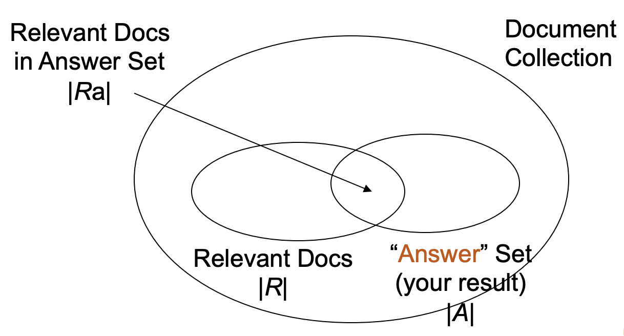
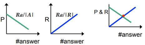
• Precision versus recall curve
  • 通常 Recall 越高，會使 Precision 越低 (tradeoff)
    • P = 100% at R = 10%
    • P = 66% at R = 20%
    • P = 50% at R = 30%

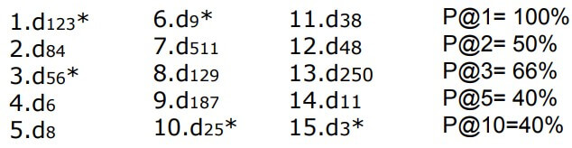
Top-k Precision (Precision at k, P@k)

• Precision evaluation in a ranking list
• The precision value of the top-k results
• Top-1 = P@1, Top-3 = P@3
• 前 5 筆有 2 筆中，P@5 = 2/5 = 40%

Top-k Precision

Average Over Multiple Queries

$$\bar{P}(r) = \frac{1}{N_q}\sum_{i=1}^{N_q}P_i(r)$$

• Average precision at the recall level r
• $N_q = \text{Number of queries used}$
• $P_i(r) = \text{Precision at recall level r for the i-th query}$

Interpolated precision

• What is interpolation mean ?
  • https://www.youtube.com/watch?v=c4_MJg_c49k

Interpolated Precision

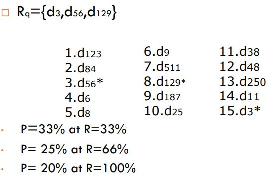
• 下方的 (P, R) 分別為讀到第三個、第八個、第十五個時候

$$P(r_i) = \max{r_i \le r \le r_{i+1}P(r)}$$

Single Value Summaries

• Average precision 可能會隱藏演算法中不正常的部分
• 需要知道對某特定 query 的 performance
• The single value should be interpreted as a summary of the corresponding precision versus recall curve

Average Precision

• Seen Relevant Documents
• obtained after each new relevant document is observed
• e.g. $(1+0.66+0.5+0.4+0.3)/5=0.57$
• 此方法對於很快找到相關文件的系統是相當有利的
  • 相關文件被排在越前面, precision 值越高

Mean Average Precision (MAP)

• Average of the precision value obtained for the top k documents
  • each time a relevant doc is retrieved
• Avoids interpolation, use of fixed recall levels

$$MAP(Q) = \frac{1}{\lvert Q \rvert} \sum_{j=1}^{\lvert Q \rvert} \frac{1}{m_j}\sum_{k=1}^{m_j}P(R_{jk})$$

R-Precision

• break-even point: recall = precision
• The precision at the R-th position in the ranking
• R : the total number of relevant documents of the current query

R-Precision

Comparison

• RNRNN NNNRR

  • MAP = (1 + 2/3 + 3/9 + 4/10) / 4 = 0.6
  • RP(4) = 2/4 = 0.5
    • (只看前四個)

• NRNNR RRNNN

  • MAP = (1/2 + 2/5 + 3/6 + 4/7) / 4 = 0.49
  • RP(4) = 1/4 = 0.25

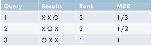
MRR: Mean Reciprocal Rank

• Rank of the first correct answer

$$MRR = \frac{1}{\lvert Q \rvert} \sum_{i=1}^{\lvert Q\rvert} \frac{1}{\text{rank}_i}$$

MRR

Precision-Recall

Class	Predicted	Correct?
orange	lemon	0
orange	lemon	0
orange	apple	0
orange	orange	1
orange	apple	0
lemon	lemon	1
lemon	apple	0
apple	apple	1
apple	apple	1

Microaveraging

• 重視數量的差距
• Each Instance has equal weight
• Largest classes have most influence

$$\text{Micro-average precision : } 4/9 =0.44$$

Macroaveraging

• 每個 rank 都一樣重要
• Each Class has equal weight

$$\begin{aligned} \text{Orange} &= 1/5 = 0.20 \\ \text{Lemon} &= 1/2 = 0.50 \\ \text{Apple} &= 2/2 = 1.00 \\\\ \text{Macro-average precision} &: (0.20+0.50+1.00) / 3 = 0.57 \end{aligned}$$

P/R 適用性

• Maximum recall 需要知道所有文件相關的背景知識
  • 平時不太可能得到標準答案，因為實際案例的 Recall 不好算
• Recall and precision 是相對的測量方式，兩者要合併使用比較適合
  • Application dependent

F-score

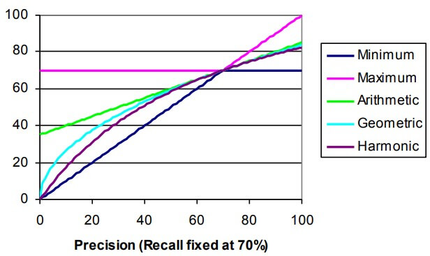
The Harmonic Mean, F-measure

$$F(j) = \frac{2}{\frac{1}{r(j)}+\frac{1}{P(j)}}, F \in [0, 1]$$

Example

F1 Examples

$$\begin{aligned} \frac{2}{\frac{1}{0.7}+\frac{1}{0.4}} &= 0.509 \\ \frac{2}{\frac{1}{0.7}+\frac{1}{0.5}} &= 0.583 \,... \end{aligned}$$

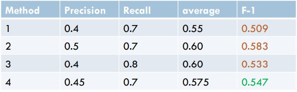
Harmonic

F1 Compare to Others

User-Oriented Measure

• 在不同領域上可以修改 recall / precision 來進行不同評分
• e.g. coverage / novelty
  • Coverage 越高，找到越多 user 期望文件
  • Novelty 越高，找到越多使用者原本不知道的文件
• 這些評分都需要先經過繁雜的 labeling

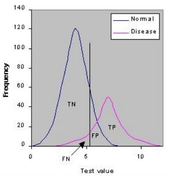
Alternative Measures (confusion matrix)

Precision Recall Table

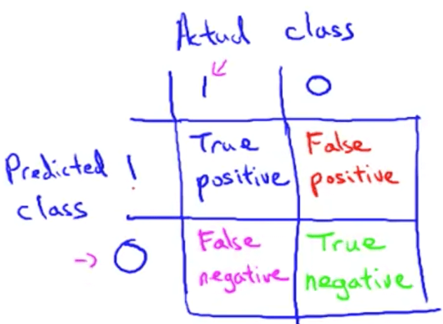
• 將預測與結果分為 True/False 的 Positive/Negative 四類
• 可以改寫原本的 Recall / Precision
  • $\text{Recall} = \frac{\lvert R_a \rvert}{\lvert R\vert} = \frac{TP}{TP+FN}$
    • Recall 又可稱為 Sensitivity
  • $\text{Precision} = \frac{\lvert R_a \rvert}{\lvert A\vert} = \frac{TP}{TP+FP}$
• 新增兩種測量方法
  • $\text{Accuracy} = \frac{TP+TN}{N}$
    • Accuracy 就是所有猜對的機率
  • $\text{Specificity} = \frac{TN}{TN+FP}$
    • Specificity 可以看作 Negative Recall
    • Not useful, TN is always too large

Example

Confusion Matrix Example

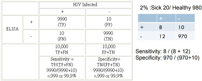
• 100% sensitivity 代表完全猜對所有生病的人
• 100% specificity 代表完全猜對所有健康的人

Limitation of Accuracy

• 想像 class 0 的 examples 有 9990 個
• 然後 class 1 的 examples 只有 10 個
• 我的模型全猜 class 0
  • Accuracy = 9990/10000 = 99.9%
  • 這個 acc 誤導我們，讓我們以為模型超強

Cost Matrix

• Cost matrix 和 confusion matrix 幾乎一樣
• 給 false negative 的 weight 加大

Example

Cost Matrix Example

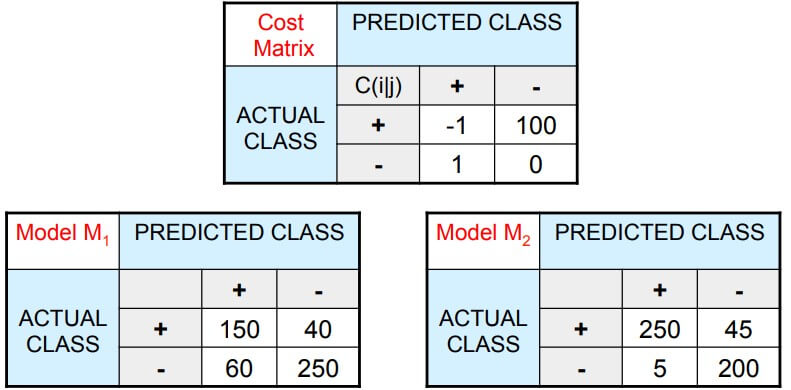
• 我們設置上面 matrix 為計算的標準
  • False Negative (猜沒生病，但其實有生病) 的權重 Cost 為 100
• 左邊的預測可以得到
  • acc = $(150+250) / (150+250+60+40) = 80\%$
  • cost = $150\times(-1) + 40\times100 + 60\times1 + 250\times0 = 3910$
• 右邊的預測可以得到
  • acc = $(250+200) / (250+200+5+45) = 90\%$
  • cost = $250\times(-1) + 45\times100 + 5\times1 + 200\times0 = 4255$
• 可以發現雖然右邊 acc 較高，但 cost 也較高
• 很多情況，例如醫學上可能就不能容許 cost 較高情況出現

ROC

• ROC : Receiver Operating Characteristic
• ROC is a plot of sensitivity vs. 1-specificity for a binary classifier

ROC

ROC curve

ROC Curve

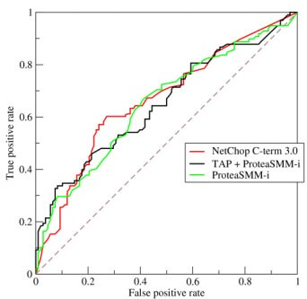
• ROC 的結果可以等同於 plot TP fraction vs. FP fraction
  • the area under the ROC curve, or "AUC"
• AUC 越大，代表分類器正確率越高

Example

ROC Curve Example

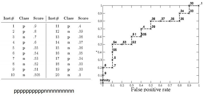
• 利用預先算好的結果 plot 到圖上
  • True Positive 就往上走
  • False Positive 就往右走
• 若是 ppppppppppnnnnnnnnnn 就會是一個 $\Gamma$ 的形狀

Issues

• ROC curves are insensitive to changes in class distribution
  • TPR and FPR are all strict columnar ratio
  • 對於不 balance 的 data，產生的結果差不多，因為是參考 ratio
• ROC measures the ability of a classifier to produce good relative scores.
  • need only produce relative accurate scores that serve to discriminate positive and negative instances

Questions

Q : What is the relationship between the value of F1 and the break-even point?

A : at break-even point F1 = P = R.

Q : Prove that the F1 is equal to the Dice coefficient of the retrieved and relevant document sets.

$$Dice(X, Y) = 2\lvert X\cap Y\rvert / \lvert X \rvert + \lvert Y \rvert$$

A :

$$\begin{aligned} P &= \frac{TP}{TP+FP} \\ R &= \frac{TP}{TP+FN} \\ F1 &= \frac{2PR}{P+R} = \frac{2TP}{2TP+FP+FN}\\\\ X &= TP+FP \\ Y &= TP+FN \\ Dice(X,Y) &= \frac{2TP}{2TP+FP+FN} \end{aligned}$$

Estimation Methods

• Holdout
  • 2/3 train, 1/3 test
• Random subsampling
  • Repeated holdout
• Cross validation
  • Partition data into k disjoint subsets
  • k-fold: train on k-1 partitions, test on the remaining one
  • LOOCV: k=n (train on all data except 1 for test)
• Stratified sampling
  • oversampling vs undersampling
• Bootstrap
  • Sampling with replacement

Evaluate Ranked list

• The ground truth is ranked / partially preferred
  • DCG
  • Correlation coefficient measurement

Discounted Cumulative Gain (DCG)

• measures the usefulness, or gain, of a document based on its position in the result list
• The gain is accumulated cumulatively
• CG is independent with the result order
• DCG is dependent with the result order
  • DCG at position p

$$DCG_p = rel_1 + \sum_{i=2}^{p}\frac{rel_i}{\log_2(i)}$$

• The $rel_i$ is the graded relevance of the result at position i

Example

Data	D1	D2	D3	D4	D5
Score	2	1	0	2	0

Higher is more relevant, The score of order above is

$$\begin{aligned} DCG_5 &= 2 + \frac{1}{\log_2(2)} + \frac{0}{\log_2(3)} + \frac{2}{\log_2(4)} + \frac{0}{\log_2(5)} \\ &= 2 + 1 + 0 + 1 + 0 \\ &= 4 \end{aligned}$$

The ideal order is 2, 2, 1, 0, 0

$$\begin{aligned} IDCG_5 &= 2 + \frac{2}{\log_2(2)} + \frac{1}{\log_2(3)} + \frac{0}{\log_2(4)} + \frac{0}{\log_2(5)} \\ &= 2 + 2 + 0.63 + 0 + 0 \\ &= 4.63 \end{aligned}$$

NDCG 將 DCG 正規化

$$NDCG_5 = \frac{DCG_5}{IDCG_5} = \frac{4}{4.63} = 0.86$$

Correlation coefficient measurement

Kendall-tau

• measure the association between two measured quantities $\frac{\text{concordant - discordant}}{\frac{n(n+1)}{2}}$
  • where $\frac{n(n+1)}{2} = \binom{n}{2}$
  • 找出所有任選兩個數字的前後關係
• e.g. Ground Truth = 12345, Result = 21534

$$\begin{aligned} \text{Concordant} &= 7 \\ &\{1, 3\}, \{1, 4\}, \{1, 5\}, \{2, 3\}, \{2, 4\}, \{2, 5\}, \{3, 4\}\\ \text{Discordant} &= 3 \\ &\{1, 2\}, \{3, 5\}, \{4, 5\}\\ \text{Kendall-tau} &= (7-3)/10 = 0.4 \end{aligned}$$

• 前後關係維持一致的是 concordant
• 前後關係變不同的是 discordant

Cohen's Kappa

• 度量兩個評分者 (rater) 的 agreement

$$\mathcal{K} = \frac{\text{Pr}(a)-\text{Pr}(e)}{1-\text{Pr}(e)}$$

Example 1

Cohen's Kappa Example

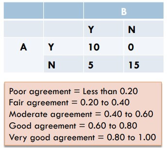
• 例如有 rater A 和 rater B
  • 在 30 個投票中，共有 25 個 agreement $\text{Agreement Pr}(a) = (10+15)/30 = 0.83$
  • 看起來很高，但有時候是因為很多 noise 導致 (例如選擇太 trivial)
  • 解決方法就是減去 $\text{Pr}(e)$ 這個 random agreement
    • 這個 $\text{Pr}(e)$ 代表的是兩人隨便亂猜就可以一致的機率

$$\begin{aligned} P(A=Y)&=10/30 = 0.33 \\ P(B=Y)&=15/30 = 0.5 \\ P(A=Y, B=Y)&= 0.33\times0.5 = 0.17 \\ P(A=N, B=N)&= 0.66\times0.5 = 0.33 \\ \Rightarrow \text{Pr}(e)&= 0.17+0.33 = 0.5 \end{aligned}$$

• 得到 a 和 e 的機率就可以算出上面的 kappa 值

$$\mathcal{K} = \frac{0.83-0.5}{1-0.5} = 0.66$$

• 所以 agreement 就從 0.83 下降至 0.66

Example 2

Cohen's Kappa Example 2

$$\begin{aligned} \text{Both Pr}(a) &= \frac{60}{100} = 0.6 \\ \text{Pr}_1(e) &= \frac{60}{100}\times\frac{70}{100} + \frac{40}{100}\times\frac{30}{100} = 0.54 \\ \text{Pr}_2(e) &= \frac{60}{100}\times\frac{30}{100} + \frac{40}{100}\times\frac{70}{100} = 0.46 \\ \mathcal{K}_1 &= \frac{0.6-0.54}{1-0.54} = 0.13 \\ \mathcal{K}_2 &= \frac{0.6-0.46}{1-0.46} = 0.26 \end{aligned}$$

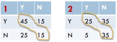
• 雖然兩題在未計算 kappa 之前的 agreement 都是 0.6
• 但計算完 kappa 後，可以發現右邊的 2 raters agreement 較好

Applicability

• each system need to use diff evaluation
  • NDCG : sort data, ranking
  • Recall : use with ground truth
  • Top-1 precision : recommendation
  • F1 : find the best in precision + recall tradeoff
  • Novelty