Introduction of Neural Networks

神經網路是為了模擬人類的大腦運作，大腦可以透過一種 learning algorithm 做到聽、說、讀、寫等活動，而神經網路的最小單位為神經元，它可以由 input wires 接收多個輸入，並將處理過的訊息傳送出去透過 output wires。我們可以再加上 bias unit 作為輸入，而處理這些 input 的為 sigmoid (logistic) activation function。當有多層 layer 時，第一層為 input layer，最後一層為 output layer，而中間所有的層統稱為 hidden layer。我們給予 hidden layer 的 nodes 一個名字：activation units，它是經由 input 和 matrix of weights 作用 output 過來的，hypothesis 就是這些 activation units 經由權重矩陣與輸入矩陣相乘後的結果。

Motivation

Motivation of Neural Networks

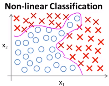
想像我們為了解決上面這個 Non-linear classification

必須使用 sigmoid function 搭配很多的 parameters 和新 features

$$g(\theta_0 + \theta_1x_1 + \theta_2x_2 + \theta_3x_1x_2 + \theta_4x_1^2x_2 + \theta_5x_1^3x_2 + \theta_6x_1x_2^2 + \cdots)$$

像上面用了兩個 features 就產生了可能 "Overfitting" 的 hypothesis

當我們有更多的 features 時，新 features 的數量將以指數成長

Example - Computer Vision

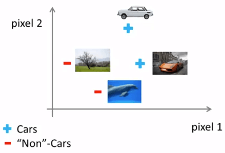
當我們要用機器學習來辨識圖片時 (舉例: 車子)

我們將整張圖片的每一個 pixel 截取出來，並給予 intensity (0-255 灰階)

我們將不同圖片的 pixel 資訊 plot 在一個二維空間中，用以分辨該 pixel 為多少時是否為車子

Computer Vision Classification

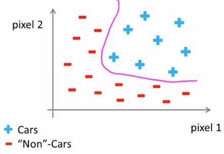
這種時候就可以用到 non-linear hypothesis

Computer Vision Classification

假設我們只要辨識 50 * 50 pixel 的小圖片

那我們將會用到 2500 的 features (7500 if RGB)

而產生的新 features 將會達到約 3 billion features

Neural Networks

一開始 neural networks 是為了試圖模擬人的大腦運作

大腦可以讓我們做幾乎任何事情，聽、說、讀、寫、看、觸 ...

而其實大腦只花了一種 learning algorithm 就做到這些事情

科學家用一種 Neural Rewiring 的實驗發現了這件事情

他們將動物接收聽覺的 Auditory Cortex REWIRE 接收視覺

他們發現 Auditory Cortex 變得能夠接收到視覺

Sensor Representation in the brain

還有許多將 Sensor 與大腦結合的發明

• 用舌頭看東西
• 人體聲納
• Haptic belt

這些東西告訴我們

其實大腦只用了一種 algorithm 來教導身體做事

而我們的最終目標就是找到這個 learning algorithm 的 hypothesis

並且把他運用在電腦上

Model Representation

Neuron

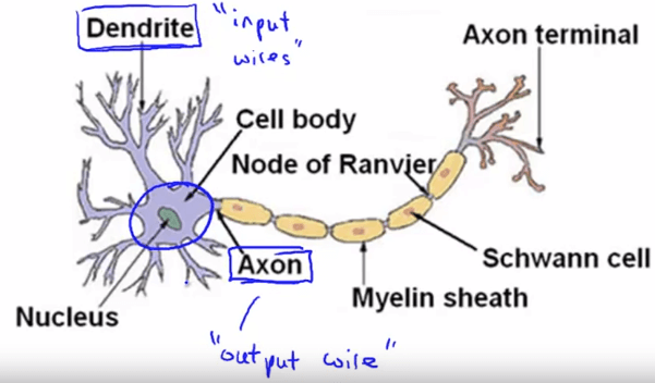
Neuron 作為 neural networks 的最小單位，模擬人類的神經元

Neuron in Human

• 透過 input wires (dendrites) 接收多個 input
• 並從 output wires (axons) 將處理過的訊息傳送出去

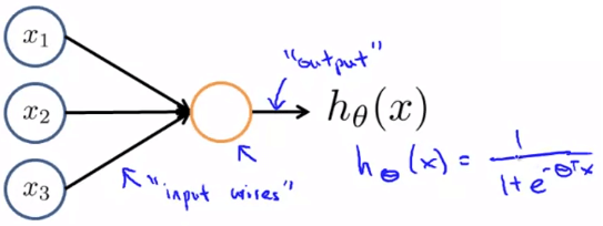Neuron in AI

其中 input 的是 features $x_1, x_2, \cdots x_n$

而 output 就是 hypothesis function $h_\theta(x)$

我們會在 input 再加上一個 $x_0$ 作為 bias unit 永遠為 1

而處理這些 input 的為 sigmoid (logistic) activation function $\frac{1}{1+e^{-\theta^Tx}}$

而在 neural networks 中 $\theta$ 這個 parameters 又稱作 "weight"

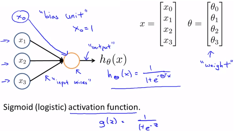Neuron in AI

當有多層 layer 時，我們稱第一層為 input layer 最後一層為 output layer

而中間所有的層統稱為 hidden layers

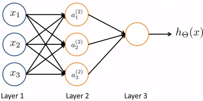3 Layers Neural Networks

Notations

我們給予上圖 hidden layer 的 nodes 一個名字: Activation units

而這些 activation units 是經由 input 和 Matrix of Weights 作用 output 過來的

$$\begin{aligned} a_i^{(j)} &= \text{activation of unit } i \text{ in layer }j\\ \Theta^{(j)} &= \text{matrix of weights controlling function mapping from layer } j \text{ to layer } j + 1 \end{aligned}$$

舉個例子來說 $a_1^{(2)}, a_2^{(2)}, a_3^{(2)}$

就是由 3x4 的 $\Theta^{(1)}$ 乘上 4x1 的 input $\vec{x}$ 向量而來

Activation Units Operation

而 hypothesis $h_\Theta(x)$ 就是

$$h_\Theta(x) = a_1^{(3)} = g(\Theta^{(2)}\vec{a}^{(2)}) = g(\Theta^{(2)}_{10}a_0^{(2)}+ \Theta^{(2)}_{11}a_1^{(2)} + \Theta^{(2)}_{12}a_2^{(2)} + \Theta^{(2)}_{13}a_3^{(2)})$$

我們可以推出 matrix of weight 的 dimension :

• 若 layer $j$ 共有 $s_j$ 個 units
• 且 layer $j+1$ 共有 $s_{j+1}$ 個 units
• 那麼 $\Theta^{(j)}$ 的 dimension 為 $s_{j+1} \times (s_j + 1)$

例如 layer 1 有 2 個 nodes 而 layer 2 有 4 個 nodes

那麼 $\Theta^{(1)}$ 的 dimension 為 4 x 3

Vectorized implementation

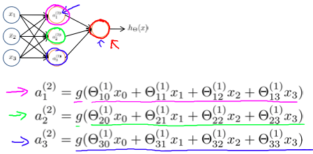
現在我們將每個 g function 內的 $\Theta$ 和 $x$ 改為矩陣運算產生的 $z$

$$\begin{aligned} a_1^{(2)} = g(\Theta_{10}^{(1)}x_0 + \Theta_{11}^{(1)}x_1 + \Theta_{12}^{(1)}x_2 + \Theta_{13}^{(1)}x_3) = g(z_1^{(2)})\\ a_2^{(2)} = g(\Theta_{20}^{(1)}x_0 + \Theta_{21}^{(1)}x_1 + \Theta_{22}^{(1)}x_2 + \Theta_{23}^{(1)}x_3) = g(z_2^{(2)})\\ a_3^{(2)} = g(\Theta_{30}^{(1)}x_0 + \Theta_{31}^{(1)}x_1 + \Theta_{32}^{(1)}x_2 + \Theta_{33}^{(1)}x_3) = g(z_3^{(2)}) \end{aligned}$$

也就是說在第 j 個 layer 的第 k 個 node，他的 z 就會是

$$z_k^{(j)} = \Theta_{k,0}^{(j-1)}x_0 + \Theta_{k,1}^{(j-1)}x_1 + \cdots + \Theta_{k,n}^{(j-1)}x_n$$

現在我們進一步將 input $x$ 向量作為 $a^{(1)}$，所以

$$\begin{aligned} z^{(2)} &= \Theta^{(1)}a^{(1)} \\ a^{(2)} &= g(z^{(2)}) \end{aligned}$$

然後 $a^{(2)}$ 必須要補個 $a_0^{(2)} = 1$ 才能繼續

$$\begin{aligned} z^{(3)} &= \Theta^{(2)}a^{(2)} \\ a^{(3)} &= g(z^{(3)}) = h_\Theta(x) \end{aligned}$$

總結來說，z 和 a 的公式如下

其中的 n + 1 為 $a_0^{(1)} = x_0, a_0^{(2)}, a_0^{(3)}, \cdots$

$$\begin{aligned} z^{(j)} &= \Theta^{(j-1)}a^{(j-1)} \text{ where } \dim({\Theta^{(j-1)}}) = s_j \times (n + 1)\\ a^{(j)} &= g(z^{(j)}) \end{aligned}$$

我們可以看到其實將最後一個 hidden layer 計算出 output layer 的過程

等同於將最後一個 hidden layer 的每個 activation units 作為 features 執行 logistic regression

而這些 activation units 其實又都是上一層的 nodes 執行 logistic regression 而來

所以這個方法稱作 Forward Propogation

意思是每一層都將計算出更有深度意義 (complex) 的 Hypothesis 至下一層

產出最好的 Hypothesis function

Applications and Intuitions

我們將使用 XNOR (NOT XOR) 的例子來解釋為何 neural networks 為何可以成功

x1	x2	XNOR
0	0	1
0	1	0
1	0	0
1	1	1

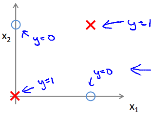XNOR classification

首先我們先來看 AND, OR 和 NOR 在 neural networks 的實作 :

AND

我們將 activation function 設成以下狀態

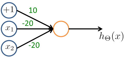
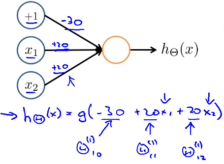AND neuron

我們知道 sigmoid function 在大於 4.6 時差不多為 1

在小於 4.6 時差不多為 0

所以我們帶進去得到

x1	x2	$h_\Theta(x)$
0	0	$g(-30) \approx 0$
0	1	$g(-10) \approx 0$
1	0	$g(-10) \approx 0$
1	1	$g(10) \approx 1$

所以這個 $h_\Theta(x)$ 可以說是 AND 的 best hypothesis

OR

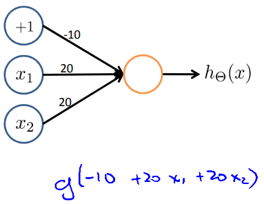OR neuron

x1	x2	$h_\Theta(x)$
0	0	$g(-10) \approx 0$
0	1	$g(10) \approx 1$
1	0	$g(10) \approx 1$
1	1	$g(30) \approx 1$

這個 Neural network 產生的 $h_\Theta(x)$ 也可以說是 OR 的 best hypothesis

NOR

首先 Negation 的 hypothesis 產生如下

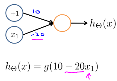Negation neuron

x1	$h_\Theta(x)$
0	$g(10) \approx 1$
1	$g(-10) \approx 0$

而 NOR 其實就是 (NOT x1) AND (NOT x2)

NOR neuron

x1	x2	$h_\Theta(x)$
0	0	$g(10) \approx 1$
0	1	$g(-10) \approx 0$
1	0	$g(-10) \approx 0$
1	1	$g(-30) \approx 0$

XNOR

現在我們有了三種 $\Theta$ for AND, OR, NOR

$$\begin{aligned} \text{AND } \Theta^{(1)} &= \begin{bmatrix} -30 & 20 & 20\end{bmatrix} \\ \text{NOR } \Theta^{(1)} &= \begin{bmatrix} 10 & -20 & -20\end{bmatrix} \\ \text{OR } \Theta^{(1)} &= \begin{bmatrix} -10 & 20 & 20\end{bmatrix} \\ \end{aligned}$$

我們將 AND 和 NOR 的 $\Theta$ 分別擺到第一層運算

而 OR 則是在最後運算

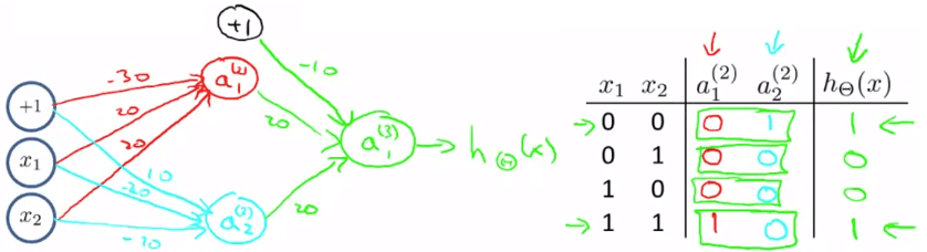XNOR neuron

$$\begin{aligned} \Theta^{(1)} &= \begin{bmatrix} -30 & 20 & 20 \\ 10 & -20 & -20 \end{bmatrix} \\ \Theta^{(2)} &= \begin{bmatrix} -10 & 20 & 20 \end{bmatrix}\\\\ a^{(2)} &= g(\Theta^{(1)} \cdot x) \\ a^{(3)} &= g(\Theta^{(2)} \cdot a^{(2)}) = h_\Theta(x) \end{aligned}$$

Multi-class Classification

現在若 Neural networks 要一次處理多種問題

例如圖片辨識需要一次辨識出 Pedestrian, Car, Motorcycle, Truck

當 training sets 為 $(x^{(1)}, y^{(1)}), (x^{(2)}, y^{(2)}), \cdots, (x^{(m)}, y^{(m)})$ 時

我們會將 y 和 hypothesis 以 vector 方式輸出

$$y^{(i)} = \begin{bmatrix}1\\0\\0\\0\end{bmatrix}, \begin{bmatrix}0\\1\\0\\0\end{bmatrix}, \begin{bmatrix}0\\0\\1\\0\end{bmatrix}, \begin{bmatrix}0\\0\\0\\1\end{bmatrix}$$

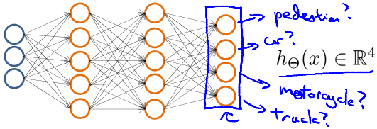Multi-class neural network

若是路人，則 $h_\Theta(x) \approx \begin{aligned}\begin{bmatrix} 1\\0\\0\\0\end{bmatrix}\end{aligned}$

若是車子，則 $h_\Theta(x) \approx \begin{aligned}\begin{bmatrix} 0\\1\\0\\0\end{bmatrix}\end{aligned}$

以此類推 ... 試圖讓 $h_\Theta(x^{(i)}) \approx y^{(i)} \mid \text{Both are } \mathbb{R}^4$