RNN Models

本文主要介紹 Gated Recurrent Unit (GRU) 和 Long Short Term Memory (LSTM) 這兩種 Recurrent Neural Network (RNN) 模型的架構及其原理。GRU 將 basic RNN 的結構加上一個 memory cell 來解決 vanishing gradients 的問題，而 LSTM 則是改進 GRU，將 basic RNN 的結構更進一步加上三個 gates 來解決 vanishing gradients 和 long-term dependency 的問題。此外，也介紹了 Bidirectional RNN (BRNN) 和 Deep RNNs (DRNN)，BRNN 能夠雙向處理句子，而 DRNN 則是將 RNN 的 hidden layers 數目增加。

Gated Recurrent Unit (GRU)

• 先回顧 basic RNN 的架構，在計算 $a^{<t>}$ 時是這樣計算 $a^{<t>} = g(W_a[a^{<t-1>}, x^{<t>}]+b_a)$
  • 可以將 basic RNN 畫成下圖表示

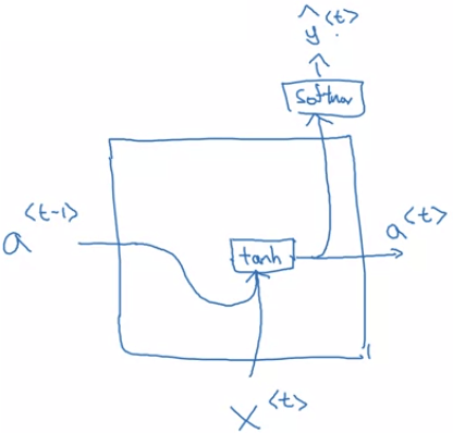Basic single RNN

• GRU 在 basic RNN 中加入一個 memory cell $(c)$ 的概念
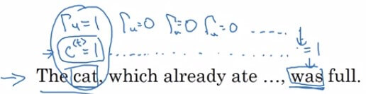
• 回到原本的句子，目標是讓網路可以記憶 cat 並在之後知道要使用 was
  • $\text{The cat, which already ate ... was full.}$
• 定義每一個 $c^{<t>}$ 會和 $a^{<t>}$ 相等 $c^{<t>} = a^{<t>}$
• 然後定義 $\tilde{c}^{<t>}$ 是可能取代掉 $c^{<t>}$ 的候補
  • $\tilde{c}^{<t>} = \text{tanh}(W_c[c^{<t-1>}, x^{<t>}]+b_c)$
• 接著定義一個 Update Gate $(\Gamma_u)$ 用來決定是否要用 $\tilde{c}^{<t>}$ 取代掉 $c^{<t>}$
  • Update Gate 最好要能 output 0/1 值，1 決定取代、0 放棄取代，所以使用 sigmoid function
  • $\Gamma_u = \sigma(W_u [c^{<t-1>},x^{<t>}]+b_u)$
• 最後用以下公式決定每個 time step 要不要更新 $c^{<t>}$
  • $c^{<t>} = \Gamma_u \times \tilde{c}^{<t>} + (1-\Gamma_u) \times c^{<t-1>}$
    • 當 $\Gamma_u = 1$ 時，後面被消掉，所以 $c^{<t>} = \tilde{c}^{<t>}$
    • 當 $\Gamma_u = 0$ 時，前面被消掉，所以 $c^{<t>} = c^{<t-1>}$

Example

RNN GRU Example

• 回到 cat 的句子問題
  • 在 cat 時把 $\tilde{c}^{<t>} = 1, \Gamma_u = 1$
    • 此時的 $c^{<t>}$ 就會被設定為 1 (假設 1 代表單數、0 代表多數)
  • 接著句子持續下去，每一個的 $\Gamma_u$ 都設定為 0，避免 cat 的資訊被刷掉
  • 直到 was 的 time step 出現，我們就可以用 $c^{<t>}$ 告訴他是 cat 要用 was
  • 等到 was 結束，不會再用到這個資訊，在之後的某個地方就會設定 $\Gamma_u = 1$ 更新
• 因為使用 sigmoid 作為 $\Gamma_u$ 的計算方式
  • 使得 $\Gamma_u$ 長期都會非常接近 0 或是 1
  • 當 $\Gamma_u = 1$ 時，$c^{<t>}$ 就會被更新
  • 當 $\Gamma_u = 0$ 時，$c^{<t>}$ 就會保持 $c^{<t-1>}$
  • 由於 c 經過很長時間依然不變，且 c 就是 a，所以也解決了 vanishing gradients

Simplified GRU

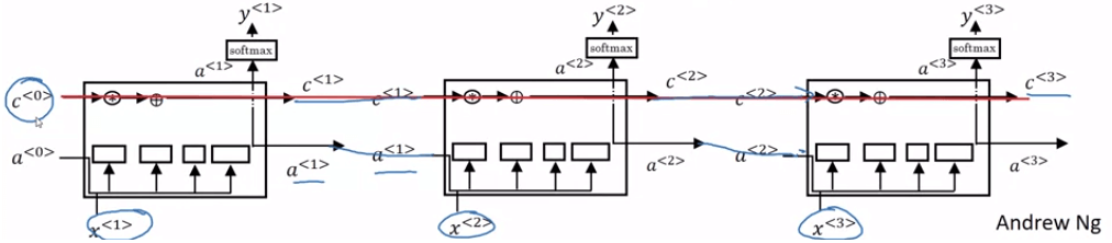
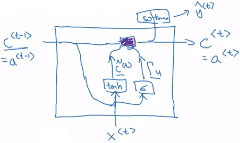Simplified GRU

• 在 GRU 的 network 中
  • 先用 $c^{<t-1>}$ 和 $x^{<t>}$ 進行 tanh 得到 $\tilde{c}^{<t>}$
  • 再用 $c^{<t-1>}$ 和 $x^{<t>}$ 進行 sigmoid 得到 $\Gamma_u$
  • 然後透過紫色區塊 (就是決定是否更新) 來更新新的 $c^{<t>} = a^{<t>}$
  • 最後跟一般一樣，產出 $\hat{y}^{<t>}$
• 要注意的是，$c^{<t>}$ 可以是一個 vector
  • 若是 $c^{<t>}$ 是一個 100 dimensional 的向量
  • 那麼 $\tilde{c}^{<t>}, \Gamma_u$ 也會是 100 dimensional
  • 而更新 $c^{<t>}$ 的乘法就會是 element-wise 的乘法 $c^{<t>} = \Gamma_u \ast \tilde{c}^{<t>} + (1-\Gamma_u) \ast c^{<t-1>}$

Full GRU

• 以上的 GRU 是簡化過的 GRU
• 在完整的 GRU 中，會再添加一個 Relevance Gate $\Gamma_r$
• Relevance gate 用來表示 $c^{<t>}$ 和 $\tilde{c}^{<t>}$ 的關聯性
• 我們在原本的 $\tilde{c}^{<t>}$
  • $\tilde{c}^{<t>} = \text{tanh}(W_c[c^{<t-1>}, x^{<t>}]+b_c)$
• 加入 Relevance gate
  • $\tilde{c}^{<t>} = \text{tanh}(W_c[\Gamma_r \times c^{<t-1>}, x^{<t>}]+b_c)$
• 而 Relevance gate 的算法也很簡單
  • $\Gamma_r = \sigma(W_r[c^{<t-1>}, x^{<t>}] + b_r)$
• Full GRU 的算式如下

$$\begin{aligned} \tilde{c}^{<t>} &= \text{tanh}(W_c[\Gamma_r \times c^{<t-1>}, x^{<t>}]+b_c)\\ \Gamma_u &= \sigma(W_u [c^{<t-1>},x^{<t>}]+b_u)\\ \Gamma_r &= \sigma(W_r[c^{<t-1>}, x^{<t>}] + b_r)\\ c^{<t>} &= \Gamma_u \times \tilde{c}^{<t>} + (1-\Gamma_u) \times c^{<t-1>} \end{aligned}$$

補充

GRU 最重要的兩篇論文 :

• Cho et al., 2014. On the properties of neural machine translation: Encoder-decoder approaches
• Chung et al., 2014. Empirical Evaluation of Gated Recurrent Neural Networks on Sequence Modeling

Long Short Term Memory (LSTM)

• LSTM 跟 GRU 長的很像，但其實 LSTM 是較早出現的架構
• LSTM 捨棄了 relevance gate，保留 update gate，並新增了 forget gate 和 output gate
  • 所以 LSTM 共有三個 gates
• LSTM 不再讓 $c^{<t>} = a^{<t>}$，並將兩者分開來計算

$$\begin{aligned} \tilde{c}^{<t>} &= \text{tanh}(W_c[a^{<t-1>}, x^{<t>}]+b_c)\\ \Gamma_u &= \sigma(W_u [a^{<t-1>},x^{<t>}] + b_u)\\ \Gamma_f &= \sigma(W_f[a^{<t-1>}, x^{<t>}] + b_f)\\ \Gamma_o &= \sigma(W_o[a^{<t-1>}, x^{<t>}] + b_o)\\ c^{<t>} &= \Gamma_u \ast \tilde{c}^{<t>} + \Gamma_f \ast c^{<t-1>} \\ a^{<t>} &= \Gamma_o \ast \text{tanh}(c^{<t>}) \end{aligned}$$

• 首先 $\tilde{t}^{<t>}$ 不再使用 $c^{<t-1>}$ 而是使用 $a^{<t-1>}$ 來跟著 $x^{<t>}$ 一起計算
• 然後依次算出 $\Gamma_u, \Gamma_f, \Gamma_o$
• 更新 $c^{<t>}$ 時，不再是兩者取一，而是將 $c^{<t-1>}$ 乘上 forget gate 後，加進 update 的 $\tilde{t}^{<t>}$
• 最終用 output gate 乘上 $\text{tanh}(c^{<t>})$ 來更新 $a^{<t>}$

LSTM nets

• 單個 LSTM 模型可以表示如下

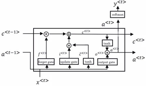LSTM Model

• 接收上一層的 $c^{<t-1>}, a^{<t-1>}$
• 結合 $x^{<t>}$ 算出三個 gate 和 $\tilde{c}^{<t>}$
• 計算出這一層的 $c^{<t>}, a^{<t>}$ 給下一層使用
• 算出預測值 $\hat{y}^{<t>}$
• 將多個 LSTM 相連在一起就是 LSTM network

LSTM Nets

Peephole Connection

• 上面的 LSTM 的三個 gate 值只有使用 $x^{<t>}, a^{<t-1>}$ 計算出來
• 但在實作上有一種方法將 $c^{<t-1>}$ 也帶入計算 gate 值
• 這種方法稱為 Peephole connection
• 注意點是，若 gate 是個 100 dimensional 的 vector
  • 那麼 c 的第 i 個值，只會影響到 gate vector 中的第 i 個值
  • 也就是 c 和 gate 的關係是 1 對 1 的
  • 跟 GRU 在更新 gate 是不一樣的

$$\begin{aligned} \Gamma_u &= \sigma(W_u[a^{<t-1>}, x^{<t>}, c^{<t-1>}] + b_u)\\ \Gamma_f &= \sigma(W_f[a^{<t-1>}, x^{<t>}, c^{<t-1>}] + b_f)\\ \Gamma_o &= \sigma(W_o[a^{<t-1>}, x^{<t>}, c^{<t-1>}] + b_o) \end{aligned}$$

Bidirectional RNN (BRNN)

• 前面也說過，單方向的 RNN 會無法處理一些問題
• 例如單字必須透過後方單字才能辨別是否是人名

$$\begin{aligned} &\text{He said, "Teddy bears are on sales!"}\\ &\text{He said, "Teddy Roosevelt was a great President!"} \end{aligned}$$

• 上面兩個句子，只讀前三個字，可能會判斷兩個 Teddy 都是人名
• 但事實上只有第二句的 Teddy 指的是人名
• 為了解決此問題，出現了能夠雙向處理的 RNN － Bidirectional RNN (BRNN)

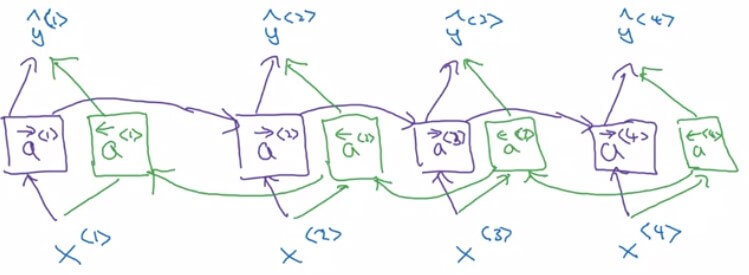Bidirectional RNN Intuition

• 為了簡化問題，假設現在只讀了前四個字 He said Teddy Roosevelt
• 首先一如往常將句子由左至右產出 $a^{<1>}, a^{<2>}, a^{<3>}, a^{<4>}$ (以 $\rightarrow$ 表示)
• 接著再將句子由右至左產出 $a^{<4>}, a^{<3>}, a^{<2>}, a^{<1>}$ (以 $\leftarrow$ 表示)
  • 要注意的是，兩個都是 forward propogation，並非 backpropogation !
• 所以現在要計算句子中任意一個 $\hat{y}^{<t>}$ 都可以配合左右兩邊的資訊來計算
  • $\hat{y}^{<t>} = g(W_y\begin{bmatrix}\overrightarrow{a}^{<t>}, \overleftarrow{a}^{<t>}\end{bmatrix}+b_y)$
• 例如要計算 $\hat{y}^{<3>}$ 的 Teddy 為人名的機率
  • $\hat{y}^{<3>} = g(W_y\begin{bmatrix}\overrightarrow{a}^{<3>}, \overleftarrow{a}^{<3>}\end{bmatrix}+b_y)$
  • 他考慮的 $\overrightarrow{a}^{<3>}$ 考慮了 a1, a2 的 He said
  • 他考慮的 $\overleftarrow{a}^{<3>}$ 考慮了 a4 的 Roosevelt
• BRNN 的缺點是需要完整的句子序列，才可以訓練並預測句子中的任意單字
• 若用在 speech recognition，不可能等所有話講完，再慢慢處理所有文字
• 所以在 speech recognition 的實際應用上，不會使用 standard BRNN
• 但是在能夠一次取得完整句子的 NLP 應用中， standard BRNN 是很有效率的

Deep RNNs (DRNN)

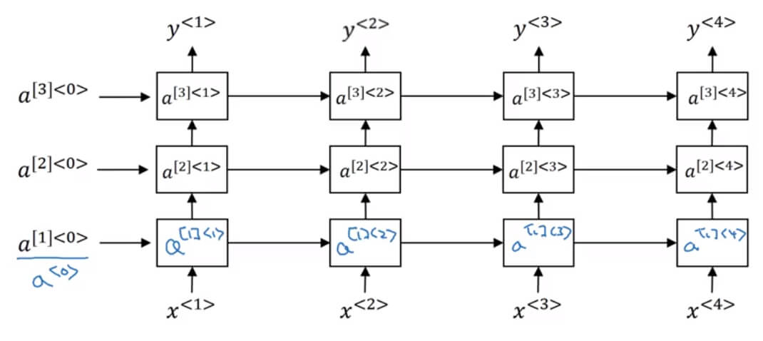Deep RNN Intuition

• 到目前為止見到的只是 one hidden layer 的 RNN model
• 事實上 RNN 也可以有多個 hidden layer，只是不會像 CNN 那麼多
• 上圖有幾個 notation 需要解釋
  • $[l]$ 用來代表第 l 層
  • $<t>$ 用來代表第 t 個 time step
  • 所以 $a^{[2]<3>}$ 代表是第 2 個 hidden layer 在第 3 個 timestep 的狀況
• 另外在 parameters 也有不同
  • $W_a^{[l]}$ 代表在第 l 層的 $W_a$
  • $b_a^{[l]}$ 代表在第 l 層的 $b_a$
  • 所以 $a^{[2]<3>}$ 的算法為 $a^{[2]<3>} = W_a^{[2]}\begin{bmatrix}a^{[2]<2>}, a^{[1]<3>}\end{bmatrix} + b_a^{[2]}$
• DRNN 中的每一個 blocks 可以是一般的、GRU、LSTM blocks
• DRNN 在計算 $\hat{y}^{<t>}$ 前，也可以先接上一連串的 fully-connected networks
• 因為 RNN 的計算量已經相當龐大，所以 DRNN 的 hidden layers 數目並不會太多