Deep neural network 是一種有較多 hidden layers 的神經網路,它能夠對輸入的資料進行複雜的運算,例如人臉辨識、語音辨識等。在一個 deep neural network 中,會使用到越來越複雜的計算,而且每一層的運算結果都會被 cache 起來給下一層使用,從而逐步把複雜的運算細分成簡單的步驟,有效的加速計算的效率。
只有 1-layer 的 logistic 及一些層數較少的 nn 會稱作 shallow neural network,而當你有越多的 hidden layers 代表你的 nn 越接近 deep neural network。
首先先介紹一些 deep neural networks 的 notation:L 表示 layer 數,n[l] 表示第 l 層的 units 有幾個,a[l] 表示第 l 層的 activations,且 a[l]=g[l](z[l]),w[l] 和 b[l] 表示 z[l] 的 weights。
x=a[0] 表示 input layer,共有 n[0](nx) 個 units;y^=a[L] 表示 output layer,共有 n[L] 個 units。
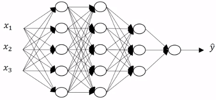 5-layer neural network
要對五層神經網路進行前向傳播,方法跟之前學的兩層很像,只是不斷對下面這個步驟迭代而已。下面是一個一般化的前向傳播步驟。
Z[l]A[l]=W[l]A[l−1]+b[l]=g[l](Z[l])X=A[0] 通常若有 l 層,就需要用 for i = 1:l 的 for-loops 而非向量化來遍歷所有層。
建置一個 nn 時,考慮好每一個 vector 及 matrix 的 dimension 是防止 program 產生問題的重點。
5-layer neural network- 先看計算第一層 z 時 w 和 b 的 dimension
z[1]=(3,1)(n[1],1)w[1](3,2)(n[1],n[0])×x(2,1)(n[0],1)+b[1](3,1)(n[1],1) - 可以一般化 w 和 b 在計算 z 時的 dimension
- 在 backprop 時,產生的 dw,db 也會和 w,b 一模一樣 dimension
w[l]b[l]=(n[l],n[l−1])=(n[l],1)=z[l] - 使用 vectorization 一次執行 m 筆 training examples 於 forward propogation 時
- 原本的 z 變成一個 m columns 的矩陣
Z[1]=⎣⎡∣z[1](1)∣∣z[1](2)∣⋯∣z[1](m)∣⎦⎤ - z 的運算變成這樣
- b 保持不變是因為 python 會自動使用 broadcasting 技巧
Z[1]=(n[1],m)W[1](n[1],n[0])×X(n[0],m)+b[1](n[1],1) - z,a 變成 Z,A 在 dimension 上就是從 1 column 變成 m columns
z[l],a[l]:(n[l],1)→Z[l],A[l]:(n[l],m) 以下用兩個方向來解釋為什麼 nn 越 deep 越好
 Deep neural network intuition
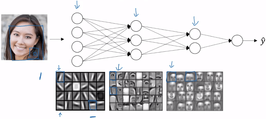
我們有了 Deep Neural Network,可以對圖片做簡單的運算和偵測,例如找出圖片的水平或垂直邊緣線。然後,我們可以組合上一層的結果,再在下一層進一步運算,例如找出五官或某個部位。越往下層走,就可以得到越複雜的計算,最後可以做到人臉辨識。
另一個例子是語音辨識系統,從 Audio 到 low level audio waves,再到 phonemes、words 和 sentences。因此,Deep Learning 能夠將一個從簡單到複雜的問題,做出近似的解決方案。
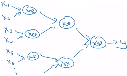
另一個例子是用邏輯電路來呈現,假設我要運算出 x1 XOR x2 XOR x3 XOR ⋯ XOR xn,一般的做法都會是使用一個 Olog(N) 的方法 (deep nn 的好處)
 Deep learning circuit theory
- 另一種 shallow 的方法則需要展開 O(2N) 的 nodes 才能做到
 Deep learning circuit theory
Informally:
- There are functions you can compute with a "small" L-layer deep neural network
- that shallower networks require exponentially more hidden units to compute.
- 在實際建置 dnn 時,可以把每一個 A[l]→A[l+1] 的 forward 想成一個 block
- 同理的,也可以將 dA[l−1]←dA[l] 的 backward 想成一個 block
- forward 會將計算好的值 cache 起來給 backward 使用
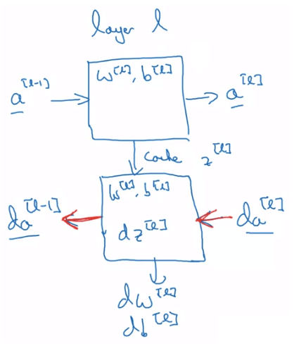 Single block of NN
- Input : a[l−1]
- Output : a[l]
- Cache : z[l],w[l],b[l]
- Process :
Z[l]A[l]=W[l]⋅A[l−1]+b[l]=g[l](Z[l]) - Input : da[l]
- Output : da[l−1],dW[l],db[l]
- Process :
dZ[l]dW[l]db[l]dA[l−1]=dA[l]⋅∗g[l]′(Z[l])=m1dZ[l]⋅A[l−1]T=m1np.sum(dZ[l])=W[l]T⋅dZ[l] 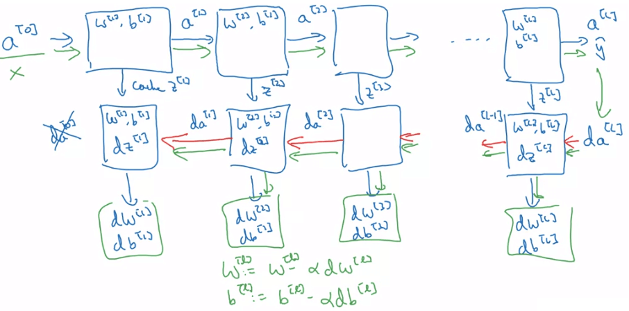 DNN blocks
一般的 parameters 是指 W[1],b[1],W[2],b[2],⋯,而 hyperparameters 指的是那些足以影響 parameters 的參數,其設定往往需要依靠著經驗,例如:
- learning rate α
- number of iterations
- number of hidden layers L
- number of hidden units n[1],n[2],⋯
- choice of activation functions tanh, ReLU,
- momentum
- mini-batch size
- regularization algorithms 等
因此 deep learning application 其實是一個非常 empirical 的過程,需要不斷的循環於 Idea -> Code -> Experiment 之間。