Model and Cost Function

Model 與 Cost Function 之間有著非常密切的關係，這是由於 Model 是用來預測的結果，而 Cost Function 則是用來計算 Model 預測結果的誤差。因此，Cost Function 將會用於最小化 Model 中出現的誤差，讓 Model 的預測結果越來越精確。

Model Representation

在監督學習 (supervised learning) 中，我們會有一些訓練集 (training sets) 來學習預測，例如用房屋大小來預測價格。

每一筆資料可以用 (x, y) 來表示，而要表達特定某一行訓練示例時可以用 (xⁱ, yⁱ)，其中 m 代表訓練示例的數量 (Number of training examples)、x's 代表輸入變數 (Input variables / features)、y's 代表輸出變數 (Output variables / features)。

Size in feet	Price in 1000
2104	460
1416	232
1534	315
...	...

$$\begin{aligned} (x^{(i)}, y^{(i)}) = \text{i}^{th} \text{ training example.}\\ \text{For example : } x^{(1)} = 2104, y^{(1)} = 460 \end{aligned}$$

所以一個 Supervised learning 的工作流程如下 :

Supervised learning workflow

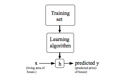
我們會將 training sets 餵進一個 learning algorithm 等他產生 output Hypothesis (h)，這個 hypothesis 是一個將 x 映射至 y 的函數，也就是我們在未來只要給定 x，hypothesis 就要能夠幫我們精準預測 y，所以接下來的重點就是如何去取得這個 hypothesis！我們首先先用簡單的線性公式來表達 hypothesis：

$$h_\theta(x) = \theta_0 + \theta_1x$$

我們可以簡寫為 $h(x)$。 將這個公式可以透過簡單的線性方程與我們 x 預測 y 的圖表結合 :

Linear regression with one variable

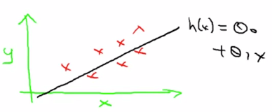
而這個簡單的模型我們稱為 Univariate linear regression (means Linear regression with one variable)

Cost Function

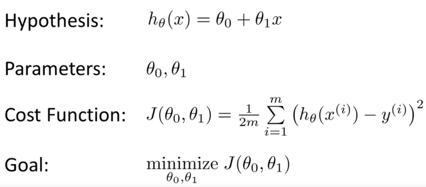
我們知道 Hypothesis 的公式為

$$h_\theta(x) = \theta_0 + \theta_1x$$

那我們要帶入什麼值給 $\theta_0$ 和 $\theta_1$，讓這個線性方程能夠最精準的預測 y 呢？這就是我們要找的 Cost function，這個 Cost function 會用來衡量 Hypothesis 的預測結果與實際結果的差異，也就是說，我們要找到一個 $\theta_0$ 和 $\theta_1$ 的組合，讓 Cost function 的值越小越好。

$$\text{Idea : Choose } \theta_0, \theta_1 \text{ so that } h_\theta(x) \text{ is close to } y \text{ for our training examples } (x, y)$$

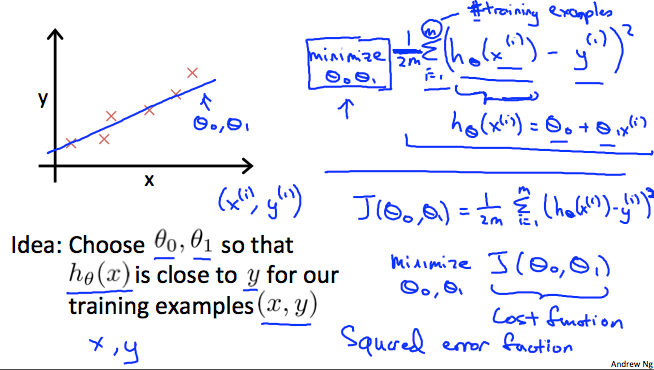
所以我們得到一個公式 (Cost function)，用於最小化 $\theta_0$ 和 $\theta_1$。 Cost function 所算出來的值越接近 0，代表越精確，其實就是在算每一個「預測的 y」和「真實的 y」的差異，平方過後並求平均值（又稱為"Squared error function"，或"Mean squared error"）。

$$J(\theta_0, \theta_1) = \frac{1}{2m} \sum_{i=1}^{m}(h_\theta(x^i)-y^i)^2$$

提示

這個 $\frac{1}{2}$ 是為了方便 gradient descent 計算，因為在微分後可以消掉這個 $\frac{1}{2}$

用圖總結一下 Cost Function :

Cost function

Intuition I

假設我們有一個非常完美的 Hypothesis (h) 被 Output 出來，這個 function 剛好是 linear equation 直線完全 fit 到所有的 training examples，所以他對應的 Cost function (J) 會是 0 才對。

備註

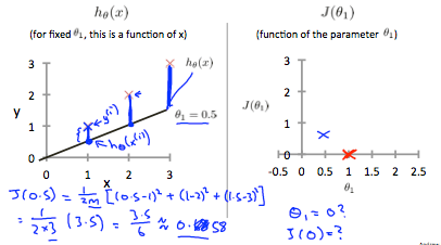
我們假設 $\theta_0$ 是 0，只要看 $\theta_1$ 就好，所以 J 會呈現一個 x, y plane。其中 x 軸代表 $\theta_1$ 的值，而 y 軸代表 Cost function 的結果。

Intuition

Intuition

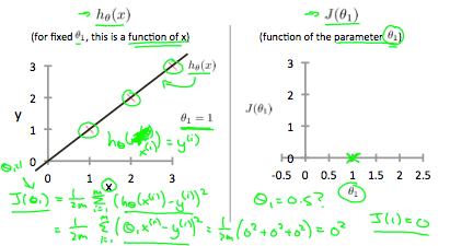
在上圖左，當 $\theta_1$ 等於 1 時，hypothesis 完全符合所有的 training sets，因此他在 cost function 中得到 0 的結果。

接著上圖右，當 $\theta_1$ = 0.5 時，Hypothesis 和每個 training sets 都有一些差距，此時他的 cost function 就等於 0.58，我們可以依此類推得出所有的 $\theta_1$，得出整個 cost function 圖表。

Cost Function with different theta 1

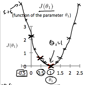
因為當 $\theta_1$ 等於 1 時，cost function 最接近（等於）0，代表誤差最小，所以我們應該要 output 一個 hypothesis，他的 $\theta_1$ 為 1，$\theta_0$ 為 0 為最佳解。

$$\begin{aligned} H_\theta(x) &= \theta_0 + \theta_1 \times x \\ &= 0 + 1 \times x \end{aligned}$$

Intuition 2

案例中我們把 $\theta_0$ 拿掉，因此 cost function 呈現為二維圖表；若 $\theta_0$ 不等於 0，cost function 就必須使用 3D 模型 (或 contour plot) 才可以視覺化。

備註

可以看到右下為 $\theta_0$，左下為 $\theta_1$，而模型最凹之處就是最小誤差的地方

Two variables cost function model

Contour 1

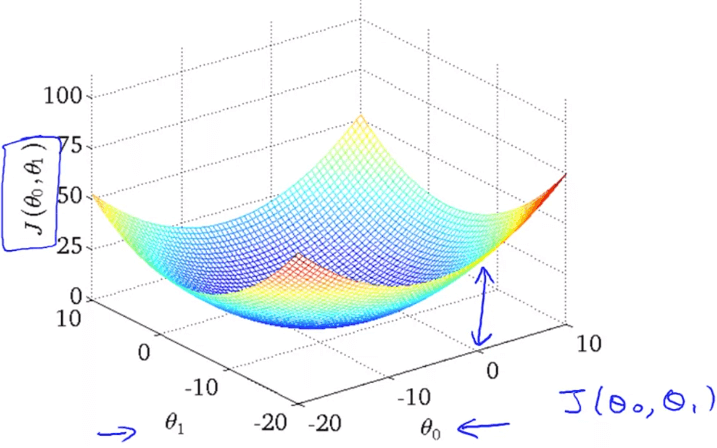
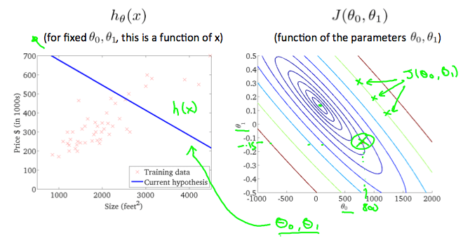
在上圖中，當 $\theta_0$ = 800 且 $\theta_1$ = -0.15 時，不用看 cost function 就知道它與真實的 training sets 有誤差，而 cost function 的值與中心點也有段距離。

而當 $\theta_0 = 250, \theta_1 = 0.12$ 時，我們可以算出他的 cost function 非常接近中心點了，也就是一個非常好的 hypothesis 了。

Contour 2

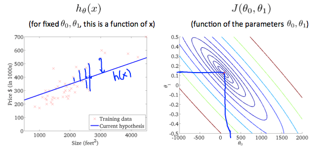
最後我們複習一下重點，也就是說要創建一個 learning algorithm，讓它自動去找出 cost function 的最低點，並且 output 出一個理想的 (Hypothesis) !

Model goal